Geospatial Visualization of Switzerland Cantons
Source:vignettes/spatial_dataviz.Rmd
spatial_dataviz.RmdThe covid19swiss dataset provides a summary of the covid19 cases in Switzerland cantons and the Principality of Liechtenstein (FL). Therefore, for the case of Switzerland cantons, it may be useful to use geospatial visualization tools to presents the data. This vignette will demonstrate how to visualize the Switzerland cantons with choropleth maps.
Note that this vignette does not include on the CRAN version due to CRNA 5mb size limitation. In addition, the following packages, that needed for this vignette, do not include in the package description and required to run this vignette:
- rnaturalearth for getting the geometric data of Switzerland cantons
- mapview for creating choropleth maps based on the Leaflet JaveScript library
- ggplot2 for creating choropleth maps
- viridisLite for color palette
To install those packages use the following code:
install.packages(c("rnaturalearth", "mapview", "ggplot2", "viridisLite"))Getting the geomatic data for Switzerland cantons
This vignette is focusing only on plotting the Switzerland cantons. Therefore, we will start by subsetting the canton data from the covid19swiss dataset, as the data also includes the Principality of Liechtenstein:
library(covid19swiss)
library(dplyr)
library(tidyr)

swiss_wide <- covid19swiss %>% filter(location != "FL",
                                      date == as.Date("2020-09-08")) %>%
  pivot_wider(names_from = data_type, values_from = value)

head(swiss_wide)
#> # A tibble: 6 x 13
#>   date       location location_type location_code location_code_t… tested_total
#>   <date>     <chr>    <chr>         <chr>         <chr>                   <int>
#> 1 2020-09-08 AG       Canton of Sw… CH.AG         gn_a1_code                 NA
#> 2 2020-09-08 AI       Canton of Sw… CH.AI         gn_a1_code                 NA
#> 3 2020-09-08 BE       Canton of Sw… CH.BE         gn_a1_code                 NA
#> 4 2020-09-08 BL       Canton of Sw… CH.BL         gn_a1_code                 NA
#> 5 2020-09-08 BS       Canton of Sw… CH.BS         gn_a1_code                 NA
#> 6 2020-09-08 FR       Canton of Sw… CH.FR         gn_a1_code                 NA
#> # … with 7 more variables: cases_total <int>, hosp_new <int>,
#> #   hosp_current <int>, icu_current <int>, vent_current <int>,
#> #   recovered_total <int>, deaths_total <int>
Note that we filter the data by using canton != "FL" to remove the Principality of Liechtenstein, and date == as.Date("2020-04-09") to take a snapshot of number of cases on April 9th, 2020.
Next, we will use the rnaturalearth package to get Switzerland geometric data, using the ne_states function:
library(rnaturalearth)
swiss_map <- ne_states(country = "Switzerland", returnclass = "sf")

str(swiss_map)
#> Classes 'sf' and 'data.frame':   26 obs. of  84 variables:
#>  $ featurecla: chr  "Admin-1 scale rank" "Admin-1 scale rank" "Admin-1 scale rank" "Admin-1 scale rank" ...
#>  $ scalerank : int  9 9 9 9 9 9 9 9 9 9 ...
#>  $ adm1_code : chr  "CHE-165" "CHE-168" "CHE-170" "CHE-171" ...
#>  $ diss_me   : int  165 168 170 171 174 176 162 3425 3423 167 ...
#>  $ iso_3166_2: chr  "CH-VS" "CH-TI" "CH-GR" "CH-SH" ...
#>  $ wikipedia : chr  NA NA NA NA ...
#>  $ iso_a2    : chr  "CH" "CH" "CH" "CH" ...
#>  $ adm0_sr   : int  1 1 1 1 1 1 1 1 1 1 ...
#>  $ name      : chr  "Valais" "Ticino" "Graubünden" "Schaffhausen" ...
#>  $ name_alt  : chr  "Vallais|Vallese|Wallis" "Tesino|Tessin" "Graubünden|Grigioni|Grischun|Grisons" "Schaffhouse|Schaffusa|Sciaffusa" ...
#>  $ name_local: chr  NA NA NA NA ...
#>  $ type      : chr  "Canton|Kanton|Chantun" "Canton|Kanton|Chantun" "Canton|Kanton|Chantun" "Canton|Kanton|Chantun" ...
#>  $ type_en   : chr  "Canton" "Canton" "Canton" "Canton" ...
#>  $ code_local: chr  NA NA NA NA ...
#>  $ code_hasc : chr  "CH.VS" "CH.TI" "CH.GR" "CH.SH" ...
#>  $ note      : chr  NA NA NA NA ...
#>  $ hasc_maybe: chr  NA NA NA NA ...
#>  $ region    : chr  NA NA NA NA ...
#>  $ region_cod: chr  NA NA NA NA ...
#>  $ provnum_ne: int  13 15 14 26 35 9 10 0 0 34 ...
#>  $ gadm_level: int  1 1 1 1 1 1 1 1 1 1 ...
#>  $ check_me  : int  20 20 20 20 20 20 20 20 20 20 ...
#>  $ datarank  : int  7 7 7 7 7 7 7 7 7 7 ...
#>  $ abbrev    : chr  NA NA NA NA ...
#>  $ postal    : chr  "VS" "TI" "GR" "SH" ...
#>  $ area_sqkm : int  0 0 0 0 0 0 0 0 0 0 ...
#>  $ sameascity: int  NA NA NA 9 NA 7 NA NA NA NA ...
#>  $ labelrank : int  9 9 9 9 9 7 9 9 9 9 ...
#>  $ name_len  : int  6 6 10 12 7 6 6 11 16 12 ...
#>  $ mapcolor9 : int  7 7 7 7 7 7 7 7 7 7 ...
#>  $ mapcolor13: int  3 3 3 3 3 3 3 3 3 3 ...
#>  $ fips      : chr  "SZ22" "SZ20" "SZ09" "SZ16" ...
#>  $ fips_alt  : chr  NA NA NA NA ...
#>  $ woe_id    : int  2347104 2347102 2347091 2347098 2347101 2347107 2347083 2347086 2347085 2347097 ...
#>  $ woe_label : chr  "Canton of Valais, CH, Switzerland" "Canton of Ticino, CH, Switzerland" "Canton of Graubunden, CH, Switzerland" "Canton of Schaffhausen, CH, Switzerland" ...
#>  $ woe_name  : chr  "Valais" "Ticino" "Graubünden" "Schaffhausen" ...
#>  $ latitude  : num  46.2 46.4 46.7 47.7 47.6 ...
#>  $ longitude : num  7.61 8.79 9.56 8.62 9.15 ...
#>  $ sov_a3    : chr  "CHE" "CHE" "CHE" "CHE" ...
#>  $ adm0_a3   : chr  "CHE" "CHE" "CHE" "CHE" ...
#>  $ adm0_label: int  2 2 2 2 2 2 2 2 2 2 ...
#>  $ admin     : chr  "Switzerland" "Switzerland" "Switzerland" "Switzerland" ...
#>  $ geonunit  : chr  "Switzerland" "Switzerland" "Switzerland" "Switzerland" ...
#>  $ gu_a3     : chr  "CHE" "CHE" "CHE" "CHE" ...
#>  $ gn_id     : int  2658205 2658370 2660522 2658760 2658372 2657895 2661876 2661602 2661603 2658821 ...
#>  $ gn_name   : chr  "Canton du Valais" "Cantone Ticino" "Kanton Graubunden" "Kanton Schaffhausen" ...
#>  $ gns_id    : int  -2554622 -2554455 -2552275 -2554062 -2554452 -2554936 -2550909 -2551185 -2551184 -2554001 ...
#>  $ gns_name  : chr  "Valais, Canton du" "Ticino, Cantone" "Graubunden, Kanton" "Schaffhausen, Kanton" ...
#>  $ gn_level  : int  1 1 1 1 1 1 1 1 1 1 ...
#>  $ gn_region : chr  NA NA NA NA ...
#>  $ gn_a1_code: chr  "CH.VS" "CH.TI" "CH.GR" "CH.SH" ...
#>  $ region_sub: chr  NA NA NA NA ...
#>  $ sub_code  : chr  NA NA NA NA ...
#>  $ gns_level : int  1 1 1 1 1 1 1 1 1 1 ...
#>  $ gns_lang  : chr  "swa" "swa" "deu" "deu" ...
#>  $ gns_adm1  : chr  "SZ22" "SZ20" "SZ09" "SZ16" ...
#>  $ gns_region: chr  NA NA NA NA ...
#>  $ min_label : num  8.7 8.7 8.7 8.7 8.7 8.7 8.7 8.7 8.7 8.7 ...
#>  $ max_label : num  11 11 11 11 11 11 11 11 11 11 ...
#>  $ min_zoom  : num  8.7 8.7 8.7 8.7 8.7 8.7 8.7 8.7 8.7 8.7 ...
#>  $ wikidataid: chr  "Q834" "Q12724" "Q11925" "Q12697" ...
#>  $ name_ar   : chr  NA NA NA NA ...
#>  $ name_bn   : chr  NA NA NA NA ...
#>  $ name_de   : chr  "Kanton Wallis" "Kanton Tessin" "Kanton Graubünden" "Kanton Schaffhausen" ...
#>  $ name_en   : chr  "Canton of Valais" "Ticino" "Graubünden" "Canton of Schaffhausen" ...
#>  $ name_es   : chr  "cantón del Valais" "Tesino" "Grisones" "Schaffhausen" ...
#>  $ name_fr   : chr  "canton du Valais" "canton du Tessin" "canton des Grisons" "canton de Schaffhouse" ...
#>  $ name_el   : chr  NA NA NA NA ...
#>  $ name_hi   : chr  NA NA NA NA ...
#>  $ name_hu   : chr  "Wallis kanton" "Ticino kanton" "Graubünden kanton" "Schaffhausen kanton" ...
#>  $ name_id   : chr  "Kanton Valais" "Kanton Ticino" "Kanton Graubünden" "Kanton Schaffhausen" ...
#>  $ name_it   : chr  "Canton Vallese" "canton Ticino" "Cantone dei Grigioni" "Canton Sciaffusa" ...
#>  $ name_ja   : chr  NA NA NA NA ...
#>  $ name_ko   : chr  NA NA NA NA ...
#>  $ name_nl   : chr  "Wallis" "Ticino" "Graubünden" "Schaffhausen" ...
#>  $ name_pl   : chr  "Valais" "Ticino" "Gryzonia" "Szafuza" ...
#>  $ name_pt   : chr  "Valais" "Ticino" "Grisões" "Schaffhausen" ...
#>  $ name_ru   : chr  NA NA NA NA ...
#>  $ name_sv   : chr  "Valais" "Ticino" "Graubünden" "Schaffhausen" ...
#>  $ name_tr   : chr  "Valais" "Ticino" "Graubünden" "Schaffhausen" ...
#>  $ name_vi   : chr  "Valais" "Ticino" "Graubünden" "Schaffhausen" ...
#>  $ name_zh   : chr  NA NA NA NA ...
#>  $ ne_id     : chr  "1159307663" "1159307671" "1159307675" "1159307677" ...
#>  $ geometry  :sfc_MULTIPOLYGON of length 26; first list element: List of 1
#>   ..$ :List of 1
#>   .. ..$ : num [1:260, 1:2] 7.85 7.85 7.85 7.85 7.84 ...
#>   ..- attr(*, "class")= chr  "XY" "MULTIPOLYGON" "sfg"
#>  - attr(*, "sf_column")= chr "geometry"
#>  - attr(*, "agr")= Factor w/ 3 levels "constant","aggregate",..: NA NA NA NA NA NA NA NA NA NA ...
#>   ..- attr(*, "names")= chr  "featurecla" "scalerank" "adm1_code" "diss_me" ...
As you can see, the se_states function returns 26 rows, one for each canton, and 84 columns. To plot the data, we will need the following variable:
-
geometry- contains the geometry data of the cantons -
gn_a1_code- the cantons code available also on the covid19swiss package, will use it as key to merge the geometry data with swiss_df -
name_en- optional, the name of the canton in English
swiss_map <- swiss_map %>%
  select(gn_a1_code, name_en)

head(swiss_map)
#> Simple feature collection with 6 features and 2 fields
#> geometry type:  MULTIPOLYGON
#> dimension:      XY
#> bbox:           xmin: 6.750368 ymin: 45.82072 xmax: 10.46663 ymax: 47.80117
#> CRS:            +proj=longlat +datum=WGS84 +no_defs +ellps=WGS84 +towgs84=0,0,0
#>     gn_a1_code                name_en                       geometry
#> 400      CH.VS       Canton of Valais MULTIPOLYGON (((7.84962 45....
#> 402      CH.TI                 Ticino MULTIPOLYGON (((8.728974 46...
#> 405      CH.GR             Graubünden MULTIPOLYGON (((9.224831 46...
#> 804      CH.SH Canton of Schaffhausen MULTIPOLYGON (((8.593589 47...
#> 805      CH.TG                Thurgau MULTIPOLYGON (((8.851935 47...
#> 806      CH.ZH       Canton of Zürich MULTIPOLYGON (((8.576305 47...
Note that the geometry is remain in the subset data we created above (even that we did not include on the select function).
Now, that we have both the canton data (swiss_wide) and geometry (swiss_map), we will merge the two using the gn_a1_code and location_code as keys:
Choropleth maps with the mapview package
Using the swiss_df object we created above, it is straightforward to create a choropleth map with mapview package. In the following example, we will use the mapview function to plot the total confirmed cases by canton. The zcol argument defines the column to display on the choropleth map:
The col.regions argument allows you to set the color palette. For instance, we can use the plasma palette from the virdisLight package to plot total death by canton:
Additional customization options can be found on the mapview package site
Choropleth maps with the ggplot2 package
Likewise, we can use the ggplot2 package to create a choropleth map with the use of the geom_sf argument:
library(ggplot2)

ggplot(data = swiss_df, aes(fill = `cases_total`)) +
  geom_sf() +
  scale_fill_viridis_b()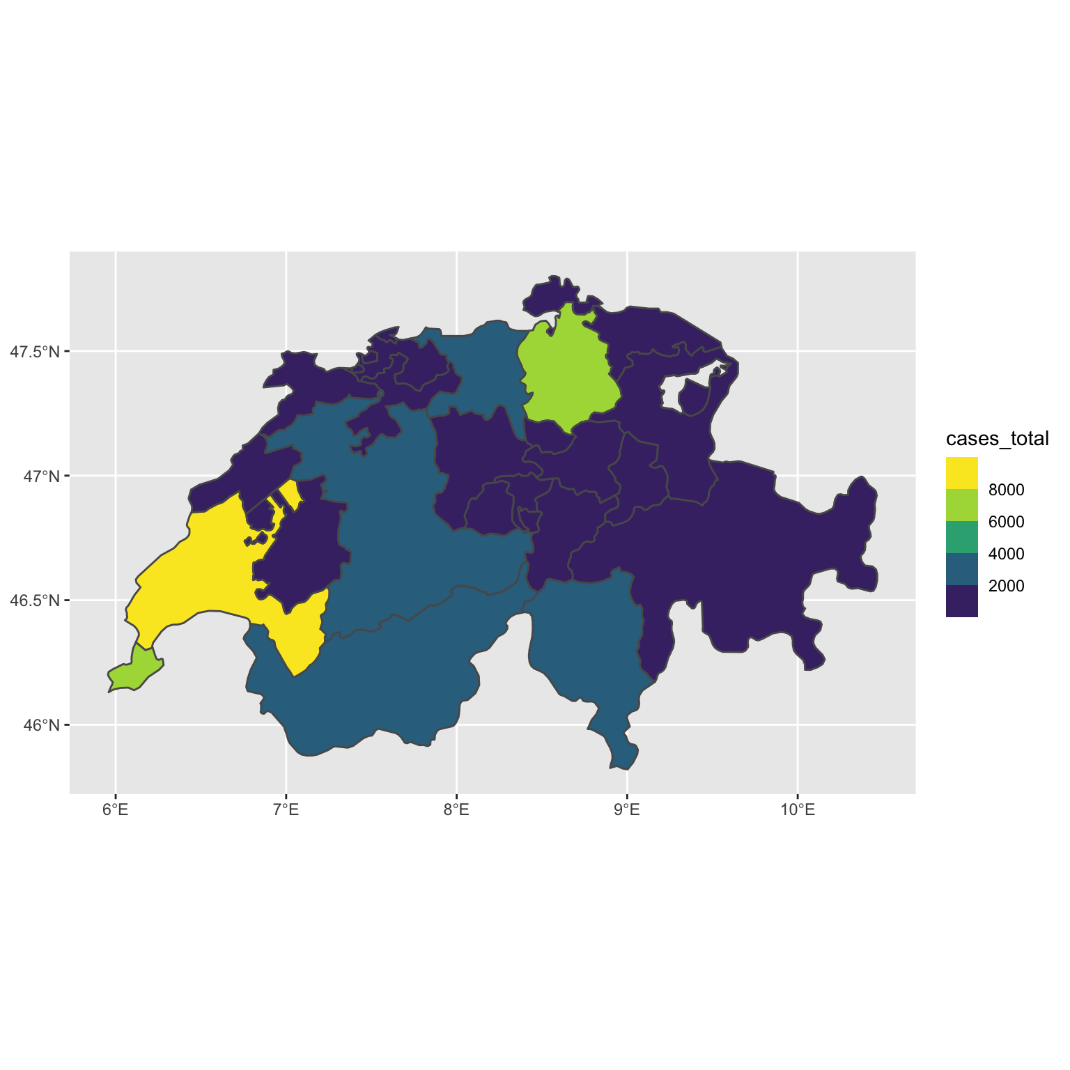
Customizations of the plot color palette can be done with the scale_fill_viridis_b function. For example, by default, the function uses the viridis palette from the viridis package. We can modify the palette to magma palette, by setting the option argument to A:
ggplot(data = swiss_df, aes(fill = `cases_total`)) +
  geom_sf() +
    scale_fill_viridis_b(option = "A",
                       begin = 0.2,
                       end = 0.7) +
   theme_void()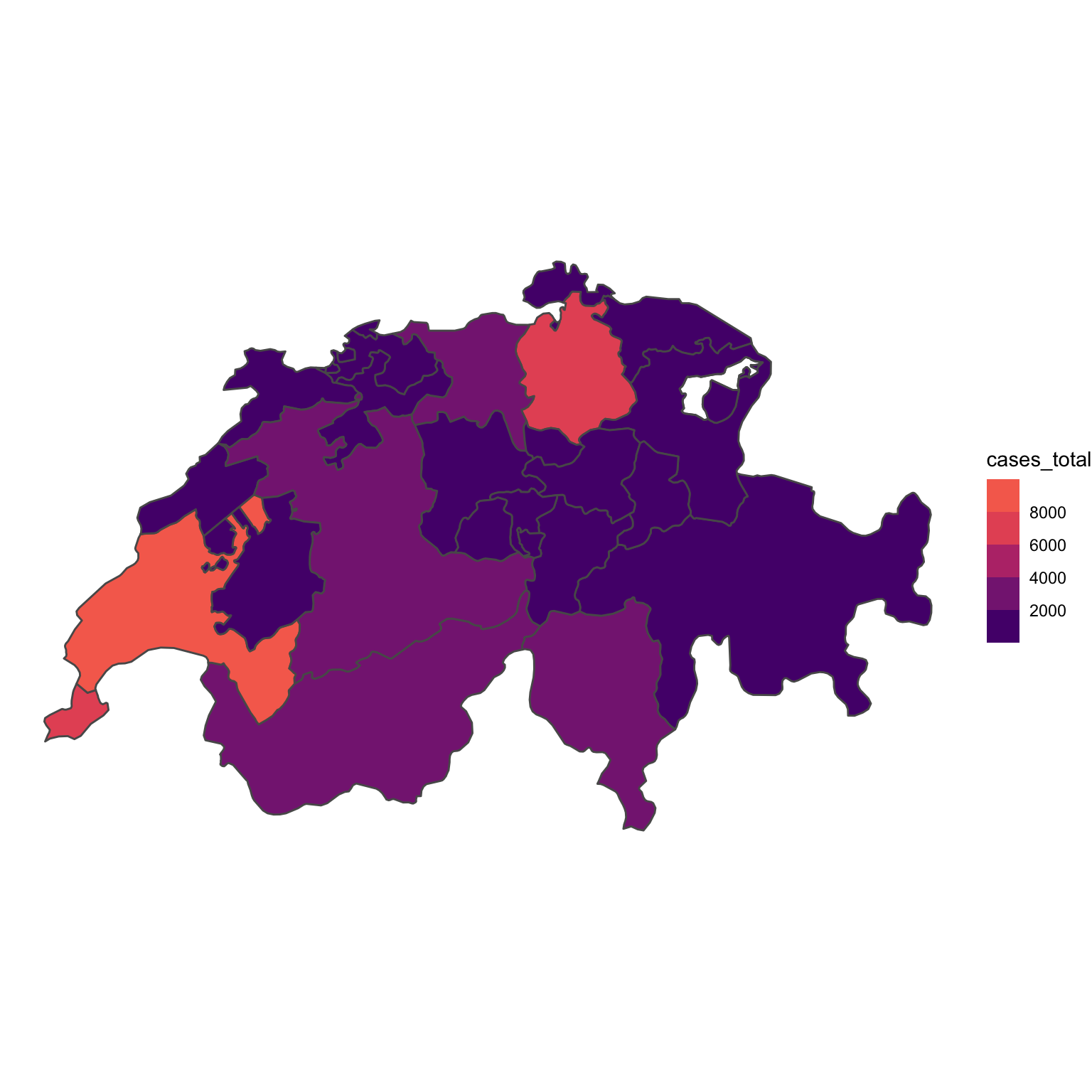
The theme_void remove the axis grids and the gray background.